Download LaTeX source Download references ENSO R code repository

After removing trends and seasonal patterns, many time series models rely on stationarity: the assumption that the statistical behavior of the data does not change over time. That assumption is powerful, but it is often unrealistic. Locally stationary basis processes provide one way to model time series whose dependence structure evolves smoothly over time.

Introduction

There is an extensive range of statistical methods for model selection, estimation, and forecasting of stationary time series. When the stationarity assumption is not appropriate, however, inference about the stochastic process of interest can be compromised.

Applications that naturally lead to nonstationary time series modeling include acoustics, biomedical science, climate science, finance, and oceanography. In these settings, local behavior may look nearly stationary even when the full time series changes over longer horizons.

Locally stationary (LS) processes have gained popularity because they can model evolving time series dependence while still allowing efficient statistical estimation. This article focuses on a subclass called locally stationary basis (LSB) processes, in which time-varying parameters are represented using smooth basis functions.

Core idea. A process can be globally nonstationary but approximately stationary over short windows. LSB processes turn this idea into a flexible modeling framework by letting model parameters evolve smoothly over rescaled time.

Locally stationary basis processes

Consider daily average temperature measured over a year in one city. The full series is nonstationary because seasonal patterns change the mean and variability. Yet, within a short window, such as a week in July, the data may behave approximately like a stationary process. Local stationarity formalizes this intuition.

Univariate locally stationary processes

To introduce LSB processes, we first recall the broader class of locally stationary processes introduced by Dahlhaus (1997). Let \(\{X_{t,T}: t=1,\ldots,T\}\) be a time series of length \(T\), and define rescaled time \(u=t/T\). This maps the time index to the interval \([0,1]\), allowing us to describe where an observation occurs proportionally within the sample.

\[X_{t,T}=\mu\!\left(\frac{t}{T}\right)+\int_{-\pi}^{\pi}\exp(i\lambda t)A^0_{t,T}(\lambda)\,dZ(\lambda).\]

Here, \(\mu(t/T)\) is a trend function that lets the mean vary smoothly over time. The transfer function \(A^0_{t,T}(\lambda)\) depends on both frequency \(\lambda\) and time, controlling how strongly each frequency contributes to the process at each time point.

\[\sup_{t,\lambda}\left|A^0_{t,T}(\lambda)-A\!\left(\frac{t}{T},\lambda\right)\right|\leq KT^{-1}.\]

This condition says that the discrete-time transfer function is close to a smooth function \(A(u,\lambda)\). As \(T\) grows, the approximation improves, which provides the smoothness needed for local stationarity.

Locally stationary basis processes

An LSB process is a locally stationary process whose time-varying transfer function can be written using a finite set of smoothly evolving parameters:

\[A(u,\lambda)=m\{\xi_1(u),\ldots,\xi_J(u);\lambda\}.\]

Each time-varying parameter curve can be represented through a generalized linear function of basis vectors:

\[g_j\{\xi_j(u)\}=w_j(u)'\beta_j.\]

The basis functions \(w_j(u)\) are smooth functions of rescaled time, such as splines, wavelets, or polynomials. The coefficients \(\beta_j\) are estimated from the data, and the link function \(g_j\) enforces model constraints. This construction is flexible while preserving properties such as local stationarity, causality, invertibility, or identifiability when appropriate.

Definition. An LSB process is a locally stationary process whose time-varying parameters are expressed with smooth basis functions. Instead of estimating a separate parameter at every time point, we estimate a smaller number of basis coefficients.

Statistical properties

Because LSB processes are a special case of LS processes and \(E\{dZ(\lambda)\}=0\), the expected value is controlled by the trend function:

\[E(X_{t,T})=\mu\!\left(\frac{t}{T}\right).\]

The time-varying spectral density function (SDF) is

\[f(u,\lambda;\beta)=|A(u,\lambda;\beta)|^2=|m\{\xi_1(u),\ldots,\xi_J(u);\lambda\}|^2.\]

At rescaled time \(u\) and frequency \(\lambda\), the SDF tells us how much variance is contributed by that frequency. It can change across both time and frequency.

The time-varying covariance function for lag \(h\) is

\[c(u,h;\beta)=\int_{-\pi}^{\pi} f(u,\lambda;\beta)\exp(ih\lambda)\,d\lambda.\]

The paper shows that this time-varying covariance function approximates the actual covariance:

\[\operatorname{cov}\{X_{[uT-h/2],T},X_{[uT+h/2],T}\}=c^0(u,h;\beta)+O(T^{-1}).\]

Application to ENSO data

El Niño and the Southern Oscillation (ENSO) is a periodic fluctuation in sea surface temperature and atmospheric pressure over the equatorial Pacific. ENSO variability often occurs on a roughly 2-to-7-year cycle. We use ENSO data to illustrate how an LSB model can capture time-varying dependence.

The functions, data, and full script are available in the ENSO_LSB GitHub repository.

Load packages and data

We begin by loading the required packages and helper functions.

library(astsa)
library(spectral)
library(fields)
library(readxl)
library(mvnfast)

source("functions/basis_functions.R")
source("functions/LSB_ARp.R")
source("functions/LSB_AR_SDF.R")

Next, load the ENSO dataset and plot the monthly index.

raw <- read_excel("data/ENSO.xlsx")

enso <- as.vector(t(as.matrix(raw[, -1])))
enso <- enso[!is.na(enso)]

T.       <- length(enso)
ts_years <- seq(1951, by = 1/12, length.out = T.)
fs       <- seq(0, 0.5, length = 128)

plot(ts_years, enso, type = "l",
     xlab = "Year", ylab = "ENSO index",
     main = "ENSO monthly index")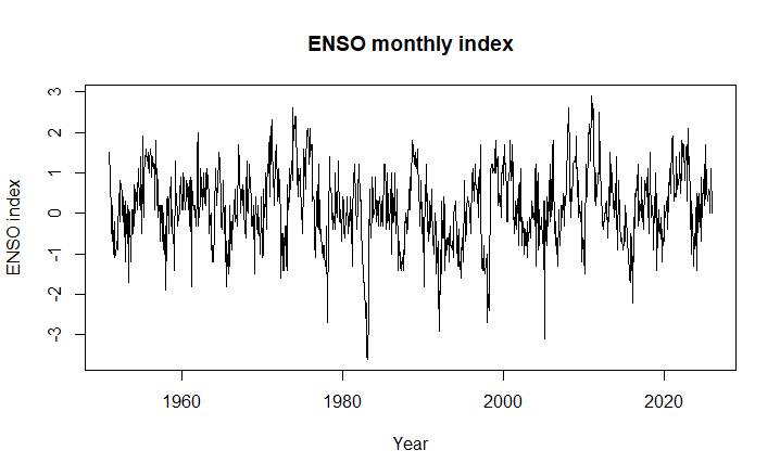

Figure 1. Raw ENSO monthly index. This plot motivates a model that allows behavior to evolve over time.

Select the model order

We fit LSB-AR(\(p\)) models with autoregressive orders \(p=2,\ldots,6\) and basis orders \(b=2,\ldots,6\). Natural cubic splines are used as basis functions, so the AR parameters change smoothly over time.

param_grid <- expand.grid(ar.order = 2:6, ar.basis.order = 2:6)

models <- mapply(
  function(p, b) LSB.ARp.model.sel(enso, p, b, X.method = "spline"),
  param_grid$ar.order,
  param_grid$ar.basis.order,
  SIMPLIFY = FALSE)

The nonstationary information criterion (NIC) and Bayesian information criterion (BIC) are extracted from each fitted model.

best_nic <- models[[which.min(sapply(models, `[[`, "NIC"))]]
best_bic <- models[[which.min(sapply(models, `[[`, "BIC"))]]

cat("NIC-selected model: AR order =", best_nic$ar.order,
    " | basis order =", best_nic$ar.basis.order, "\n")
cat("BIC-selected model: AR order =", best_bic$ar.order,
    " | basis order =", best_bic$ar.basis.order, "\n")

Using NIC, we select an LSB-AR(3) model with basis order 2 for the AR parameters. We then choose the number of basis functions for the time-varying variance.

b_values   <- 2:6
var_models <- lapply(b_values, function(s)
  LSB.ARp.model.sel(enso, best_nic$ar.order, best_nic$ar.basis.order,
                    s = s, X.method = "spline"))

best_s <- b_values[which.min(sapply(var_models, `[[`, "NIC"))]
cat("Variance basis order:", best_s, "\n")

Two basis functions are selected for the variance curve. We then fit the LSB-AR(3) model with two basis functions for the AR parameters and two for the variance.

p <- best_nic$ar.order
b <- best_nic$ar.basis.order
s <- best_s

build_basis <- function(orders) {
  lapply(orders, function(d)
    build.X(n = T., X.deg = d, X.method = "spline"))
}

fit_lsb <- function(basis_orders, ...) {
  X <- build_basis(basis_orders)
  fit <- optim(
    rep(0.01, sum(basis_orders + 1)),
    LSB.ARp.lik,
    y = enso, X = X,
    method = "L-BFGS-B", ...
  )
  list(fit = fit, X = X)
}

tv  <- fit_lsb(c(rep(b, p), s), hessian = TRUE)  # time-varying
sta <- fit_lsb(rep(0, p + 1))                    # stationary

Time-varying spectral density

After fitting the model, we compute the time-varying spectral density function.

the.beta   <- theta.to.beta.list(tv$X, tv$fit$par, p)
the.phi    <- beta.list.to.phi.list(tv$X, the.beta, p)
the.sigma2 <- eta.to.sigma2(calc.eta(tv$X[[p + 1]], the.beta[[p + 1]]))

ar.sdfs <- lapply(seq_len(T. - p), function(k)
  dB(ar.sdf(freqs  = fs,
            phi    = as.vector(the.phi[[p]][1:p, k]),
            sigma2 = the.sigma2[k])))

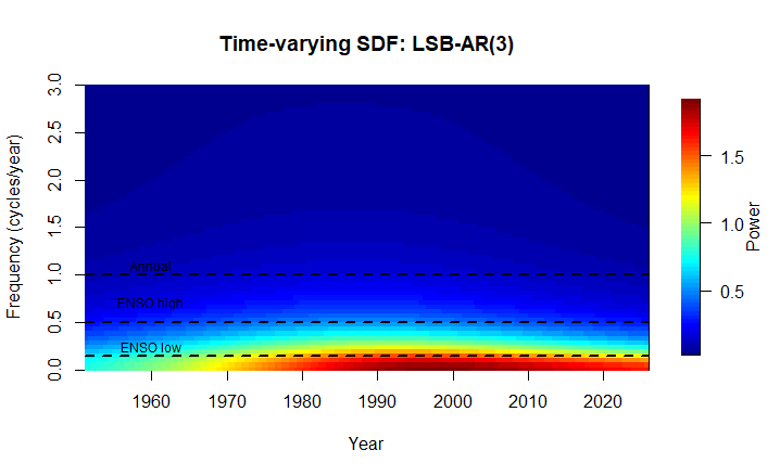
sp.matrix <- t(sapply(ar.sdfs, identity))

Decibel note. The plotted SDF values use a decibel transformation through dB(...). This log-scale transformation makes differences in spectral power easier to see visually. Figures 2 and 3 use the dB scale; Figure 4 shows the corresponding non-dB versions for comparison.

The spectral matrix is displayed as a heat map. Frequency is converted from cycles per month to cycles per year by multiplying by 12. This makes the ENSO band, roughly 2 to 7 years, and the annual cycle easier to interpret.

image.plot(
  ts_years[(p + 1):T.],
  fs * 12,
  sp.matrix,
  xlab = "Year",
  ylab = "Frequency (cycles/year)",
  main = paste0("Time-varying SDF: LSB-AR(", p, ")"),
  ylim = c(0, 3)
)
abline(h   = c(1/7, 1/2, 1), lwd = 2, lty = 2)
text(x      = 1960,
     y      = c(0.25, 0.75, 1.1),
     labels = c("ENSO low", "ENSO high", "Annual"),
     cex    = 0.75)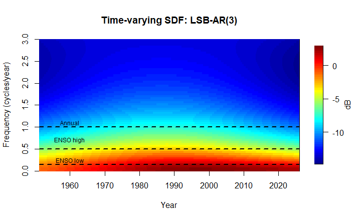

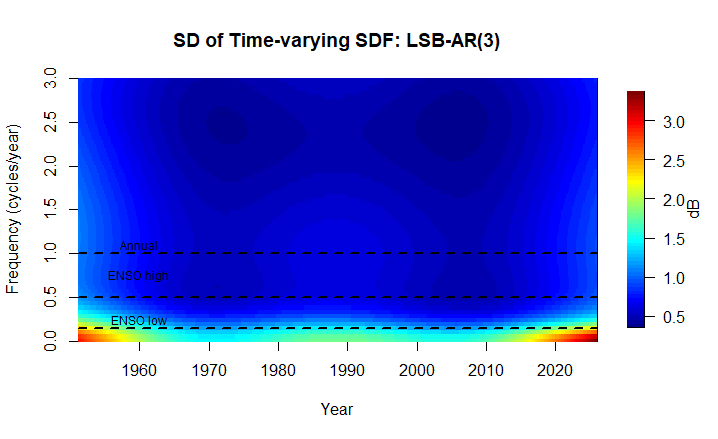
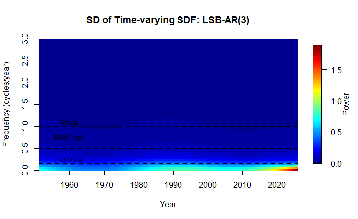
Figure 2. Time-varying SDF of the ENSO series using the decibel transformation. The dashed lines mark the ENSO and annual frequency ranges.

We can also quantify uncertainty by simulating from the estimated parameter covariance matrix and computing the standard deviation of the time-varying SDF.

cov.mat <- solve(tv$fit$hessian)

par.sim <- mvnfast::rmvn(
  1000,
  mu    = tv$fit$par,
  sigma = cov.mat
)

sdfs <- lapply(1:nrow(par.sim), function(i)
  LSB.ARp.sdf(par = par.sim[i, ], X = tv$X, fs = fs))

spec.sd <- array(
  sapply(1:(nrow(sdfs[[1]]) * ncol(sdfs[[1]])), function(x)
    sd(unlist(lapply(sdfs, "[[", x)))),
  dim(sdfs[[1]])
)

Figure 3. Standard deviation of the time-varying SDF using the decibel transformation.

Figure 4a. Time-varying SDF without the decibel transformation.

Figure 4b. Standard deviation of the time-varying SDF without the decibel transformation.

Testing stationarity

As a formal check, we test whether the nonstationary LSB model provides a significantly better fit than a stationary AR model of the same order.

test_stat <- -2 * (tv$fit$value - sta$fit$value)
df        <- sum(c(rep(b, p), s)) - (p + 1)
p_value   <- pchisq(test_stat, df = df, lower.tail = FALSE)

cat(sprintf("Stationarity test: statistic = %.2f, df = %d, p-value = %.4f\n",
            test_stat, df, p_value))

The stationarity test yields a p-value of 0.0498. At the 5% significance level, this suggests evidence against stationarity. In the time-varying SDF, the dominant frequency range expands over time, suggesting that the ENSO cycle has become more frequent and stronger. Flexible nonstationary models such as LSB processes are useful for describing this type of evolving behavior.

Glossary

Time series

A sequence of data points indexed in chronological order, such as \(\{y_t:t=1,2,\ldots,n\}\).

Weakly stationary process

A finite-variance process whose mean is constant over time and whose autocovariance depends only on the lag between two time points.

Locally stationary process

A process that is nonstationary globally but behaves approximately like a stationary process within short local windows.

Locally stationary basis process

A locally stationary process whose time-varying parameters are defined using a small number of smooth basis functions.

Transfer function

A function that describes how different frequencies contribute to a stochastic process at a specific point in time.

Spectral density function

A function that describes how the variance of a time series is distributed across frequencies.

Basis functions

Elementary functions such as splines, wavelets, or polynomials used to represent smooth curves with a finite number of coefficients.

Link function

A function that maps linear predictors to constrained parameter ranges.

ENSO

El Niño and the Southern Oscillation, a coupled ocean-atmosphere fluctuation in the equatorial Pacific.

References

1. Dahlhaus, R. (1997). Fitting time series models to nonstationary processes. The Annals of Statistics, 25(1), 1-37.
2. Ganguly, S., & Craigmile, P. F. (2025). Modeling nonstationary time series using locally stationary basis processes. Journal of Time Series Analysis.
3. Shumway, R. H., & Stoffer, D. S. (2025). Time Series Analysis and Its Applications: With R Examples. Springer.
4. McPhaden, M. (2025). Has climate change already affected ENSO? NOAA Climate.gov.
5. NOAA National Centers for Environmental Information: ENSO monitoring.